Sheet 3.2: Transformer configurations & Training utilities#
Author: Polina Tsvilodub
This sheet introduces a few more architectural details that occur in the context of language models, and briefly mentions some engineering details that are often used when training LMs. Specifically, the learning goals for this sheet are:
understand the concept of different model heads
learn to choose the head appropriate for you needs
gain a conceptual overview of a few popular engineering “tricks” needed for stable training of LMs
see a practical example of ‘masking’ used for training masked language models like BERT.
Model heads#
So far, when using a language model, we have been using models intended for next-token prediction. In other words, we have been using models whose last layer outputs a distribution over the vocabulary, from which we choose the next token. This last model layer is sometimes called the model head; therefore, so far we’ve been using models with a language modeling head.
For instance, we used GPT-2 either by loading it with the AutoClass:
from transformers import AutoModelForCausalLM

gpt2 = AutoModelForCausalLM.from_pretrained("gpt2")
or via a specific class, namely, GPT2LMHeadModel:
from transformers import GPT2LMHeadModel

gpt2 = GPT2LMHeadModel.from_pretrained("gpt2")
In the former case, the AutoClass lets HF figure out the architecture automatically based on a config file that is downloaded when the model is downloaded from HF based on the name “gpt2”.
The special class is provided specifically for GPT-2. Note that both classes provide a hint as to which task we want to initialize the model for. The AutoClass name includes CausalLM, meaning that the class will initialize a model with a next-token prediction head, and the GPT-2 class name includes LMHead directly, also meaning that a next-token prediction head will be initialized.
However, it is common in NLP to use the same architectures with different model heads for different tasks. For instance, based on the core of GPT-2, instead of next-token prediction, we might want to do classification or, e.g., token classification. For these tasks, we need different output layers (rather than one outputting a distribution over the vocabulary), i.e., different model heads. The base architecture (e.g., GPT-2) is often called the model backbone (also in computer vision).
Luckily, HF provides different classes for different model heads. For instance, for GPT-2 there are classes like GPT2ForSequenceClassification or GPT2ForTokenClassification.
The full list of different GPT-2 classes with different heads can be found here.
Note that different model head choices entail different training objectives, i.e., potentially one has to use different loss functions or different labels.
For instance, GPT2ForTokenClassification could be used for POS tagging or a named-entity-recognition (NER) task. For the latter, for instance, we could consider the task of extracting city names and person’s names, so for each token, we’d want to assign one of the three labels: [CITY] (0), [PER] (1), [NONE] (2). Therefore, during training, the inputs would be tokens, and the labels would be numbers corresponding to the correct labels. The output layer needs to assign a distribution over the possible labels for each token; this is done by a nn.Linear layer outputting scores (3 scores in this example).
Since this is a classification task where each token has only one correct category, the CrossEntropy (classification) loss is used for training.
Information about the layer and the loss can be found, e.g., when inspecting the source of the class.
Exercise 3.2.1: Model heads
Inspect the documentation for
GPT2ForSequenceClassificationhere. (1) What kind of layer is under the hood of “ForSequenceClassification”? (2) What kind of loss should be used to train a model for sequence classification?One popular task in NLP is extractive question answering. Conceptually, it refers to the task of predicting the location of a passage of text preceding a question which contains the answer to that question. Here is the class implementing such a system with GPT-2. Inspect it, perhaps search for other resources, so as to get a conceptual understanding what this task looks like. Then, for yourself, identify what a model trained for extractive QA should output when given the following input: “The quick brown fox jumped over the lazy brown dog. Who did the fox jump over?” (assume word-wise tokenization)
For yourself, for each of the following tasks, select one or several possible model heads from the list of GPT-2 heads that you think work best for the task:
POS tagging
sentiment classification
summarization
multiple-choice question answering
translation
Click below to see the solution.
It has another linear layer which takes the representation of the last token in the sequence and predicts a class. The number of nodes in this layer depends on the nuber of classes we want to predict. For the loss function we have to distinguish three cases:
We have only one class (sentiment analysis with continuous values between -1 and 1): MSE loss
We have multiple classes but only one class can be assignes to a given input (e.g. sentiment analysis, negative, positive, neutral): Cross Entropy loss
We have multiple classes and multiple classes can be assigned to a given input (e.g. topic classification, a sequence can have multiple topics): Binary Cross Entropy loss with logits loss
It would probably generate “lazy brown dog”, because it determines a span with the relevant tokens and outputs a start and end index.
POS tagging: GPT2ForTokenClassification
sentiment classification: GPT2ForSequenceClassification
summarization: GPT2LMHeadModel
multiple-choice question answering: GPT2DoubleHeadsModel
translation: GPT2LMHeadModel
Training utilities#
Training deep neural networks with millions of parameters is a tricky task. The last decades of NLP research have identified (mostly by testing what works well in practice) several engineering tricks that usually help to stabilize the optimization process. The following (non-exhaustive!) list provides an overview of commonly used tricks, so as to equip you with a high-level conceptual idea of what these are when you encounter them in NLP papers:
Learning rate scheduling: refers to using a schedule for decreasing the learning rate that is used for updating the weights. Helps to avoid too large updates close to potential optima.
Weight / gradient clipping: refers to setting min or max values that a single weight or a gradient can take on. Helps to avoid very large values in the updates of the weights or in loss computations.
Weight initialization: when training a NN from scratch, the weights are first initialized with some values. There are various ways of doing so, for instance:
Zero initialization: all weights to zero
Random initialization: weights with random values (often sampled from a standard normal distribution)
He initialization: multiplying the random initialization with \(\sqrt{\frac{2}{n}}\), where n is the size of the previous layer.
Hyperparameter tuning: refers to generally selecting configurations of the model and / or the training process. For instance, it can be the process of searching for optimal learning rates, optimal dimension of hidden representations, number of layers, etc. To avoid having to test too many combinations of hyperparameters (as in an exhaustive algorithm such as grid search), specialized algorithms have been developed that balance exploration and convergence. A few common approaches include:
Grid search: defines a list of values for each parameter and tries all possible combinations, while evaluating the models performance for each combination.
Random search: Samples values randomly from a specified distribution and again, evaluates the performance for each combination.
Bayesian Optimization: Defines an objective function \(P(score | hyperparameters)\) and tries to maximize this probability. It is essentially another machine learning model trained to find the optimal hyperparameters. The advantage to the other two approaches is that it makes an informed guess based on previous observations.
Exercise 3.2.2: Training tricks
Find out what cosine learning rate scheduling is (as a high-level concept), how to use it in PyTorch, and write a few lines of code that could be added to the model in sheet 2.4 to use it in training.
Click below to see the solution.
The learning rate is dynamically changed during training. It starts with a certain value defined by the user and decreases over epochs until a certain minimum is reached. After that it increases again until it reaches the initial value again. The changes of the learning rate follow the cosine function. The benefit is that it has a higher change to find the minimum in respect to the loss.
Interpreting training dynamics#
Lastly, an important part of training a model is being able to understand whether it is actually successfully learning. There are different ways of doing so. For instance, we could stop the training every now and then and test the model on our desired task, and check if it performs the task correctly on a held out test set. Since we want to quantify the quality of the performance, we might compute a test accuracy (if applicable for the task). Alternatively, we could look at the test loss. Another possibility of checking training progress is to rely on the training loss which should decrease with successful training.
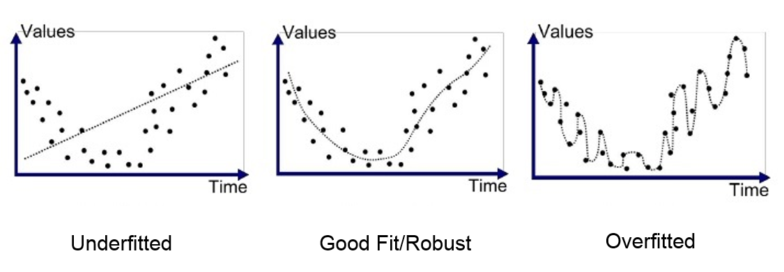
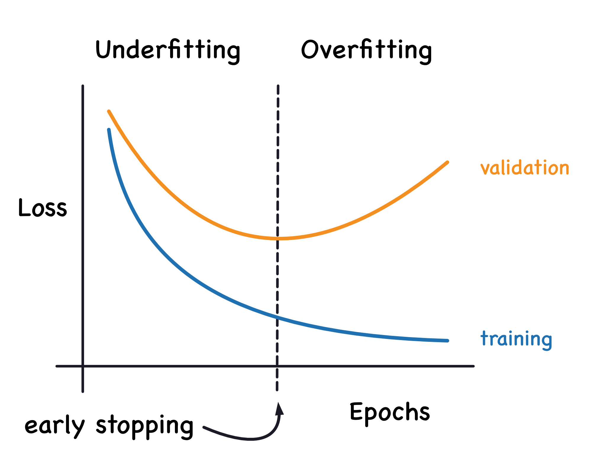
In practice, both of these things are done in combination in model training loops (e.g., see HW1 ex. 3). Commonly, both training and test (or, validation) losses are plotted and inspected over the training epochs. This is done to avoid overfitting – the issue arising when the model starts to “memorize” the training set (i.e., does very well on it), at the cost of generalizing to other data set. This can be identified when the training loss further decreases while the validation loss starts to increase.

Source here
The image illustrates the models predictions as the dotted line and the actual training data as points. The subplots show different stages of model fit. The first plot shows underfitting, i.e., the model failed to learn the data pattern at all. The middle plot shows ideal generalization. The last plot shows that the model is fitted too tightly to the training set and fails to capture the general pattern in the training data. The model’s performance on a test set which exhibits the same general pattern but will have slightly differently distributed datapoints will be worse.
In order to get the model at its “ideal” fitting and generalization stage (or as closely as possible to it), often, the training and validation losses are plotted against each other and so-called early-stopping is applied. This refers to stopping the model training as soon as the validation loss start increasing and diverging from the training loss (or, model weights saved at the respective epoch are used). The image below illustrates this.

Source here
MLM masking#
A different type of masking than what we have seen for causal language modeling are masks used with masked language models like BERT. Here, the objective is to predict a single masked token (or, even spans of multiple tokens in other models) based on the entire rest of the sequence. During training, usually tokens are masked at random at a certain rate (e.g., 0.15 in BERT). For the sentence “The quick fox jumped.”, for instance, the actual training input could be “The quick [MASK] jumped.”, and the training labels would be “The quick fox jumped.”.
The helper class DataCollatorForLanguageModeling(tokenizer, mlm=True, mlm_probability=0.15) that we’ve used in the previous sheet allows to flexibly switch between the different types of masking via the mlm parameter:
# If you are using Colab, you may have to install datasets again
# !pip install datasets
from transformers import DataCollatorForLanguageModeling
from datasets import load_dataset
from transformers import AutoTokenizer


dataset = load_dataset("stanfordnlp/imdb", split="train")
bert_tok = AutoTokenizer.from_pretrained("bert-base-cased")
data_collator = DataCollatorForLanguageModeling(bert_tok, mlm=True, mlm_probability=0.45)

def tokenize(
        input_text,
        max_length=64,
        tokenizer=bert_tok
    ):
    """
    Function to tokenize text into a series of input ids.

    Arguments
    ---------
    input_text : the text to tokenize.
    max_length : the maximal number of resulting tokens.
    tokenizer  : instantiated tokenizer of a masked LM.

    Returns
    -------
    input_ids corresponding to the tokenized text and an attention_mask,
    where padding tokens are masked.
    """
    tokenized_input = tokenizer(
        input_text["text"],
        max_length=max_length,
        padding="max_length",
        truncation=True,
        return_tensors="pt"
    )
    # mask padding tokens so that the model doesn't attend to them
    # more on masking next week
    tokenized_input["attention_mask"] = (tokenized_input["input_ids"] != tokenizer.pad_token_id).long()
    return {"input_ids": tokenized_input['input_ids'],
            "attention_mask": tokenized_input['attention_mask']}

tokenized_datasets = dataset.map(
    tokenize, batched=True, remove_columns=dataset.column_names
)
subsampled_dataset = tokenized_datasets.select(range(10))
# inspect what masked inputs for MLM look like
out = data_collator([subsampled_dataset[i] for i in range(3)])
for key in out:
    print(out)
##Note: Masking DataCollatorForMLM will return a “label” tensor in which 85% of the item are of value [-100] . This is because when we compute loss during pre -training, we want to compute it in relation to the words the model was tasked with retrieving (the 15% “masked” part of the output), and not include the others in the calculation. This type of masking is not to be confused with attention masking:
attention masking ensures that the model does not attend to things like padding tokens, or prevents a causal model from accessing the right side of the input, during the specific step of attention computing
label masking, such as the one in DataCollator, ensures that some tokens are not included in the loss computation. There are cases where we would want the token to attend to tokens like CLS or SEP (so they are accessible during the attention computation), but do not include them in the loss calculation.
Outlook and optional exercises#
The following part contains optional resources and exercises that you could work on if you’d like to practice programming more.
Here are a few additional resources that cover useful topics for training LLMs:
this tutorial exemplifies what to do when training texts exceed the maximal context size of the LM.
this tutorial provides another example of a sequence-to-sequence model, this time, tuned to do summarization (while the lecture examples covered sequence-to-sequence machine translation). The tutorial uses a popular seq2seq architecture, T5.
Exercise 3.2.3: Optional exercises
Implement the character-level name generation model from sheet 2.4, but now use an LSTM cell instead of an RNN cell.
Re-implement the model from ex. 3 of HW1 as an extractive question answering model (rather than a generative question answering system).
To see an example implementation of a character based bidirectional LSTM see here


